Visualizing an AOI location with GGPlot
Ronja Seitz
2025-07-10
About this tutorial
Here you can find a quick tutorial how to create an overview map of an Area of Interst (AOI) on Svalbard with a Digital Elevation Model (DEM) as basemap.
The final plot can be saved and used in presentations, reports etc.
1. Setup packages
Install required packages
This is only necessary once, when the packages have never been installed before.
#install.packages("terra")
#install.packages("sf")
#install.packages("ggplot2")
Load required packages
These are the packages that are needed to create the maps
library(terra) #process raster data
library(sf) #process vector data
library(ggplot2) #create plots
2. Download and load DEM
A DEM is usually a large file therefore it has to be downloaded on you personal laptop for this tutorial. Here we use the DEM of Svalbard provided by the Norsk Polar institude. You can download it here.
# input data
dem_path <- "C:/Users/ronja/Documents/EAGLE/Svalbard/Data/Basemap/NP_S0_DTM20/S0_DTM20.tif" #path to dem

# load input data
dem_raster <- rast(dem_path) #Load DEM using the Terra package.
3. Create aoi layer
For our AOI we create a bounding box indicating the corners of our area of interest (AOI). We have to assign a coordinate system matching the one of the DEM. The coordinate system most commonly used in Svalbard is UTM zone 33N, so we define this first and assign it to the bounding box of our AOI.
# Define UTM zone and bounding box (Example: UTM Zone 33N)
utm_zone <- 33  # Change based on your location
utm_crs <- paste0("+proj=utm +zone=", utm_zone, " +datum=WGS84 +units=m +no_defs")

# Define bounding box for bjorndalen in UTM (Easting, Northing)
utm_bbox <- st_sfc(st_polygon(list(matrix(c(
  505000 , 8676038,  # Bottom-left (E, N)
  509000 , 8676038,  # Bottom-right (E, N)
  509000 , 8684990,  # Top-right (E, N)
  505000 , 8684990, # Top-left (E, N)
  505000 , 8676038  #close polygon
), ncol = 2, byrow = TRUE))), crs = utm_crs)
4. Create a map of the AOI on Svalbard
We can first map Svalbard without the AOI.
To save processing time we crop the DEM to the exact extent of Svalbard, as well as aggregate it so reduce the resolution by the factor 5.
Note: GGplot only uses dataframes as input so we
create a new variable with as.data.frame().
# Aggregate using mean (for continuous data)
# Define the cropping extent (xmin, xmax, ymin, ymax)
crop_extent <- ext(xmin(dem_raster), 775254 , 8473192, ymax(dem_raster))  # Define exact extent Svalbard

# Crop the raster
r_cropped <- crop(dem_raster, crop_extent) #crop the DEM to the extent defined earlier
r_agg <- aggregate(r_cropped, fact = 5, fun = mean) #aggregate pixels of DEM to reduce resolution and decrease processing time
dem_df <- as.data.frame(r_agg, xy = T)
Now we plot! More infos about ggplot and plotting rasters can be
found here.
You can change parameters like
scale_fill_viridis_c(option = "E") or title and axis
labeling.
gg_map_svalbard <- ggplot(data = dem_df) +
  geom_raster(aes(x = x, y = y, fill = S0_DTM20)) +
  scale_fill_viridis_c(option = "E") +
  theme_light() +
  theme(legend.position = "right") +
  labs(
    title = "DEM of Svalbard",
    x = "Longitude",
    y = "Latitude"
  ) +
  coord_sf(crs = st_crs(25833))

gg_map_svalbard
At last we add our AOI to the map that we just created and we can use
ggsave() to save it as a image file.
gg_map_svalbard_box <- gg_map_svalbard +
    geom_sf(data=utm_bbox, colour = "red", fill = NA)

gg_map_svalbard_box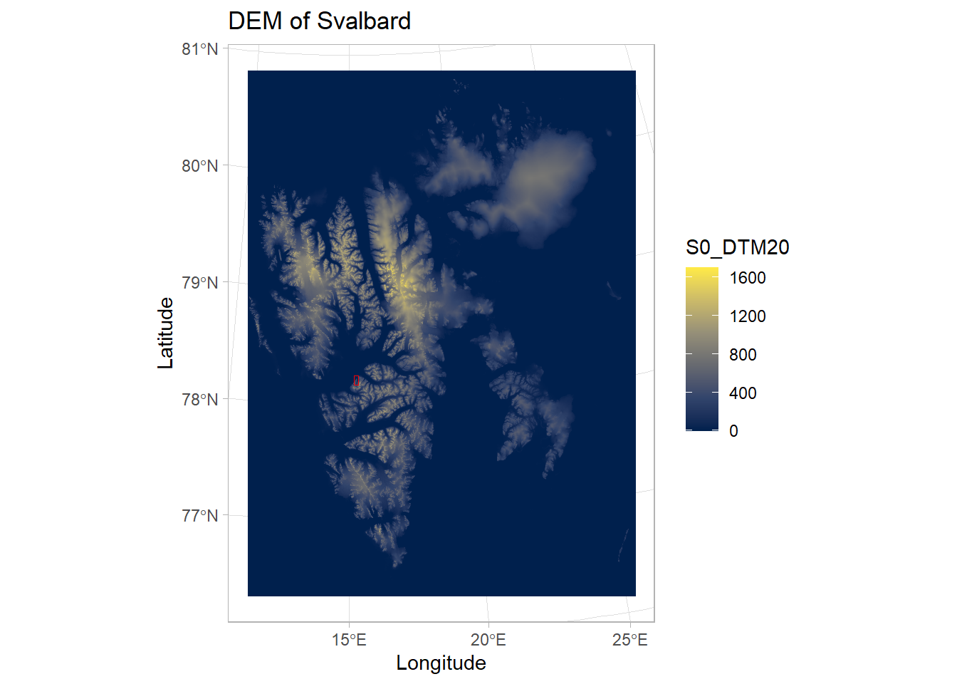
ggsave("gg_map_svalbard_box.png", plot = gg_map_svalbard_box, width = 8, height = 6, dpi = 300)Using the function sessionInfo() gives insight into the
R version, platform, packages and local settings to increase
reproducibility and is good practice to include at the end of
scripts.
sessionInfo() ## R version 4.4.1 (2024-06-14 ucrt)
## Platform: x86_64-w64-mingw32/x64
## Running under: Windows 11 x64 (build 22631)
##
## Matrix products: default
##
##
## locale:
## [1] LC_COLLATE=German_Germany.utf8 LC_CTYPE=German_Germany.utf8
## [3] LC_MONETARY=German_Germany.utf8 LC_NUMERIC=C
## [5] LC_TIME=German_Germany.utf8
##
## time zone: Europe/Berlin
## tzcode source: internal
##
## attached base packages:
## [1] stats graphics grDevices utils datasets methods base
##
## other attached packages:
## [1] ggplot2_3.5.1 sf_1.0-18 terra_1.7-83
##
## loaded via a namespace (and not attached):
## [1] sass_0.4.9 generics_0.1.3 class_7.3-22 KernSmooth_2.23-24
## [5] digest_0.6.36 magrittr_2.0.3 evaluate_1.0.1 grid_4.4.1
## [9] fastmap_1.2.0 jsonlite_1.8.8 e1071_1.7-16 DBI_1.2.3
## [13] viridisLite_0.4.2 scales_1.3.0 codetools_0.2-20 textshaping_0.4.0
## [17] jquerylib_0.1.4 cli_3.6.3 rlang_1.1.4 units_0.8-5
## [21] munsell_0.5.1 withr_3.0.2 cachem_1.1.0 yaml_2.3.10
## [25] tools_4.4.1 dplyr_1.1.4 colorspace_2.1-1 vctrs_0.6.5
## [29] R6_2.5.1 proxy_0.4-27 lifecycle_1.0.4 classInt_0.4-10
## [33] ragg_1.3.3 pkgconfig_2.0.3 pillar_1.10.1 bslib_0.8.0
## [37] gtable_0.3.6 glue_1.7.0 Rcpp_1.0.12 systemfonts_1.1.0
## [41] xfun_0.49 tibble_3.2.1 tidyselect_1.2.1 highr_0.11
## [45] rstudioapi_0.17.1 knitr_1.48 farver_2.1.2 htmltools_0.5.8.1
## [49] rmarkdown_2.29 labeling_0.4.3 compiler_4.4.1