Creating 3D Maps with Rayshader
Ronja Seitz
2025-07-04
About this tutorial
Here you can find a quick tutorial how to create 3D maps from a Digital Elevation Model (DEM). This example creates a map of Bjørndalen and adds point locations of reindeer to the 3D map.
Keep in mind that 3D maps are a good method to visualize data, however they are often not scientific. So think about for which purpose you create this map.
For more tutorials check the rayshader website or look online.
Note: This website is only capable of automatically generatic 2D figures. All 3D images are screenshots. When using these examples in R Studio the 3D maps are interactive.
1. Setup packages
Install required packages
This is only necessary once, when the packages have never been installed before.
#install.packages("terra")
#install.packages("sf")
#install.packages("rayshader")
#install.packages("magick")
#install.packages("tidyverse")
Load required packages
The creation of 3D plots is an advanced way of visualising data. Therefore there are multiple packages need:
- terra: For working with raster data
- sf: For working with vector data
- rayshader: For visualization of elevation data in 2D and 3D
- magick: For working with image data
library(terra)
library(sf)
library(rayshader)
library(magick)
library(tidyverse)
2. Load and crop DEM
The main input data for the visulaization is a DEM, here we use the DEM of Svalbard provided by the Norsk Polar Institude. You can download it here.
We use rast() to load the .tif file. It is usually a
very big file so the first thing is that we crop it to the extent that
we need - here Bjørndalen via a bounding box.
Then we create a simple figure using the base R function
plot() and save the cropped raster to a new file with the
terra function writeRaster().
# Load DEM from Norsk Polar institute
dem_path <- "/Users/ronja/Documents/EAGLE/Svalbard/Data/Basemap/NP_S0_DTM20/S0_DTM20.tif" #create a variable with the link to the DEM
dem_raster <- rast(dem_path) #load the DEM as spatial raster file into R

# Define coordinate system (crs) for the bounding box (UTM Zone 33N)
utm_zone <- 33
utm_crs <- paste0("+proj=utm +zone=", utm_zone, " +datum=WGS84 +units=m +no_defs")

# Define bounding box (all 4 corners)for bjorndalen in UTM coordinate system
utm_bbox <- st_sfc(st_polygon(list(matrix(c(
  505000, 8676038,
  509000, 8676038,
  509000, 8684990,
  505000, 8684990,
  505000, 8676038
), ncol = 2, byrow = TRUE))), crs = utm_crs)

# Crop DEM to bounding box
dem_bjorndalen <- crop(dem_raster, utm_bbox)

#plot a simple figure of the cropped DEM in grey color scale
plot(dem_bjorndalen, main = "Digital Elevation Model of Bjørndalen",
     col = gray.colors(1000, start = 0, end = 1),
     xlab = "Easting", ylab ="Northing")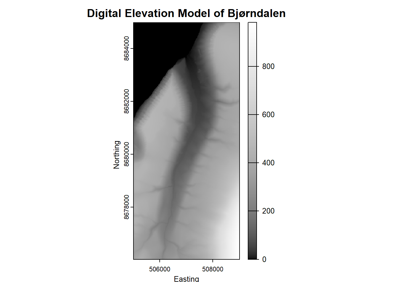
#save this cropped raster file to a folder
writeRaster(dem_bjorndalen, "data/bjorndalen_dem.tif", overwrite = TRUE)
3. Prepare DEM for use in Rayshader
To use the DEM with rayshader it has to be tranformed into a
matrix (raster_to_matrix()). Then the rayshader function
sphere_shade() is used to create a shaded relief which is
used to plot both a 2D plot (plot_map()) and a 3D plot
(plot_3d()).
You can change the title text or play around with the scaling of the 3D plot.
# Convert DEM to matrix
dem_bjorndalen <- rast("data/bjorndalen_dem.tif")
bjorndalen <- raster_to_matrix(dem_bjorndalen)

# Create shaded relief. "Desert" is an example but you can find more textures in the internet.
bjorndalen_shade <- sphere_shade(bjorndalen, texture = "desert")

# 2D map
plot_map(bjorndalen_shade,
         title_text = "Bjørndalen Shiny\n Elevation Map",
         title_size = 20)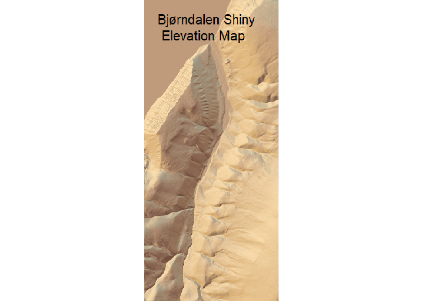
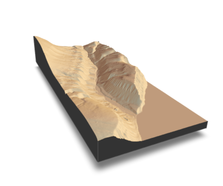
# 3D map (run in RStudio)
plot_3d(bjorndalen_shade, bjorndalen, zscale = 15, fov = 60, theta = 45, phi = 45)
This image is a screenshot of the 3D map created before. Use the code on your personal computer to create an interactive 3D map and change the scaling parameters.
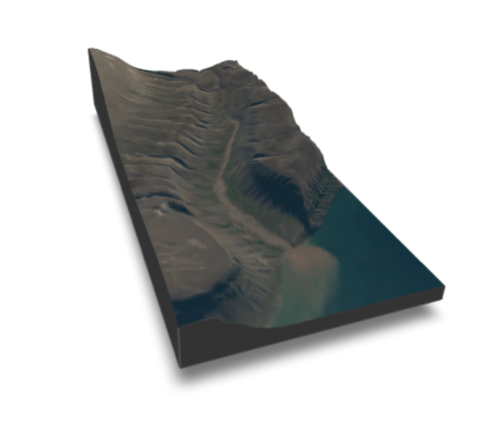
4. Load, crop and overly an orthophoto in Rayshader
Now we want to have an orthophoto as overlay for the 3D image. For this I used the Satellittbildemosaikk av Svalbard (Sentinel2, 2020) by the Norsk Polar institute and cropped it to the Bounding box. You can download the cropped image from the linked github repository or do the same as before, when cropping the DEM to the Bounding Box.
# Load orthophoto using the magick package and preprocess the image
orthophoto <- image_read("data/Ortophoto_Bjorndalen.tif") %>% #read the image
  image_resize(paste0(ncol(bjorndalen), "x", nrow(bjorndalen))) %>%  #resize to match dimensions of dem
  image_data() #convert into 3D array with RGB channel for the use in rayshader

orthophoto_rgb <- drop(as.numeric(orthophoto)) #convert to numeric format

bjorndalen_ortho_shade <- rayshader::add_overlay(bjorndalen_shade, orthophoto_rgb) #create an overlay of an RGB image on top of a hillshade terrain model

# 3D map with RGB overlay
plot_3d(bjorndalen_ortho_shade, bjorndalen, zscale = 15, fov = 60, theta = 45, phi = 45)
This code created a 3D figure with a RGB overlay. Try it in your own code to inspect it more closely!
5. Visualize reindeer locations
The final step is to visualize some reindeer locations. For this add
points as a geopackage (.gpkg) via the vect() function.
Then crop it to the extent of our area of interest (AOI)
(crop()).
data_points <- vect("data/BjorndalenReindeer_Points.gpkg") #add reindeer locations from a point file
data_cropped <- crop(data_points, dem_bjorndalen) #crop the files to the extent that we are looking at (crop point to raster)
# Extract coordinates because we need them as separate variables
coords_x <- geom(data_cropped)[, c("x")]
coords_y <- geom(data_cropped)[, c("y")]
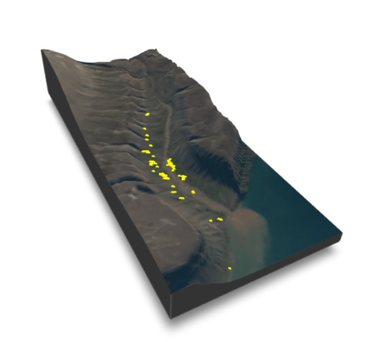
# Add 3D points and render them on our 3D plot of Bjorndalen
render_points(lat = coords_y, long = coords_x,
heightmap = bjorndalen,
zscale = 15, color = "yellow",
extent = ext(dem_bjorndalen),
offset = 1,
clear_previous = TRUE,
size = 5)The result is a final map which shows the locations of reindeer observations in Bjørndalen.
What do you think? Are the results plausible? Where were the most sightings of reindeer?
Using the function sessionInfo() gives insight into the
R version, platform, packages and local settings to increase
reproducibility and is good practice to include at the end of
scripts.
sessionInfo() ## R version 4.4.1 (2024-06-14 ucrt)
## Platform: x86_64-w64-mingw32/x64
## Running under: Windows 11 x64 (build 22631)
##
## Matrix products: default
##
##
## locale:
## [1] LC_COLLATE=German_Germany.utf8 LC_CTYPE=German_Germany.utf8
## [3] LC_MONETARY=German_Germany.utf8 LC_NUMERIC=C
## [5] LC_TIME=German_Germany.utf8
##
## time zone: Europe/Berlin
## tzcode source: internal
##
## attached base packages:
## [1] stats graphics grDevices utils datasets methods base
##
## other attached packages:
## [1] lubridate_1.9.4 forcats_1.0.0 stringr_1.5.1 dplyr_1.1.4
## [5] purrr_1.0.2 readr_2.1.5 tidyr_1.3.1 tibble_3.2.1
## [9] ggplot2_3.5.1 tidyverse_2.0.0 magick_2.8.5 rayshader_0.38.11
## [13] sf_1.0-18 terra_1.7-83
##
## loaded via a namespace (and not attached):
## [1] gtable_0.3.6 xfun_0.49 bslib_0.8.0 htmlwidgets_1.6.4
## [5] tzdb_0.4.0 vctrs_0.6.5 tools_4.4.1 generics_0.1.3
## [9] parallel_4.4.1 rgl_1.3.17 proxy_0.4-27 highr_0.11
## [13] pkgconfig_2.0.3 KernSmooth_2.23-24 lifecycle_1.0.4 compiler_4.4.1
## [17] progress_1.2.3 munsell_0.5.1 codetools_0.2-20 htmltools_0.5.8.1
## [21] class_7.3-22 sass_0.4.9 yaml_2.3.10 rayimage_0.15.1
## [25] pillar_1.10.1 crayon_1.5.3 jquerylib_0.1.4 classInt_0.4-10
## [29] cachem_1.1.0 iterators_1.0.14 foreach_1.5.2 tidyselect_1.2.1
## [33] digest_0.6.36 stringi_1.8.4 fastmap_1.2.0 grid_4.4.1
## [37] colorspace_2.1-1 cli_3.6.3 magrittr_2.0.3 base64enc_0.1-3
## [41] e1071_1.7-16 withr_3.0.2 prettyunits_1.2.0 scales_1.3.0
## [45] timechange_0.3.0 rmarkdown_2.29 png_0.1-8 hms_1.1.3
## [49] evaluate_1.0.1 knitr_1.48 doParallel_1.0.17 rlang_1.1.4
## [53] Rcpp_1.0.12 glue_1.7.0 DBI_1.2.3 rstudioapi_0.17.1
## [57] jsonlite_1.8.8 R6_2.5.1 systemfonts_1.1.0 units_0.8-5